If you have not yet visited it, look at Jack Ord's site for more simulations.

Simulating motion in one, two and three dimensions.

1D ( one dimensional) motion

We will need to know what was happening at the start of our investigation, viz. where our test object was, and how fast it was moving.

Initial Conditions

    y           =   0                   '   initial displacement
    vy          =   0                   '   initial velocity
    t           =   0                   '   initial time
    dt          =   0.001               '   time interval between updates

We will now be able to keep working out what happens a small time dt later, using the definitions of velocity and acceleration. You need to work consistently in one set of units- most scientists will choose the mks system, with distance in metres, velocity in m s^-1; acc'n in m s^-2 and forces in Newtons.

'Recipe' to step forward in time

[start]
    accn    =F /m                        '  Newton's Second Law
    vy      =vy +accn *dt                '  since accn     =vel'y change /time interval
    y       =y  +vy   *dt                '  since velocity =pos'n change /time interval
    t       =t  +dt                      '  ie time moves on a step of dt
    if still in range, goto [start] and repeat.

This is a loop which we go round, stepping forward by a step dt in time which is small enough to create only small changes in the other variables. The results can be a table; exported as csv; or, best, displayed as a graph. This is quite the easiest way to see what is happening.

A way to see the results.

This may involve printing values as a table; exporting them as csv for a graphic or spreadsheet application; graphing within Basic; or animated diagrams.

Case 1- 1D, F =0

If initial v was zero, nothing is going to happen however long we wait!

If initial v was non-zero, we'll just keep coasting along at the same velocity for ever, in the same direction. The displacement will increase linearly.

Click 'refresh' to watch it again!

Case 2 -1D, F exists, and is constant and along the line of motion.

Velocity will steadily increase ( or decrease), which we call 'uniform acceleration'. Displacement v. time will follow a parabolic curve. This is provable by very simple calculus, but can be demonstrated by the numerical stepping forward method, usually referred to as 'numerical integration'.

'Initial conditions
    x           =   0                   '   initial horizontal position. Try changing to say 10.
    vx          =   0                   '   try changing this to say 5 m s^-1.
    t           =   0                   '   initial time.
    dt          =   1                   '   time interval between updates. ( Use .001 to slow it down.)
    force       =   1                   '   constant, forward force. Try changing this to 0.
    mass        =   1                   '   mass of moving object.

  [here]
    print t, x, vx, accnx
'The calculation loop
    accnx   =force /mass
    vx      =vx +accnx *dt
    x       =x     +vx *dt
    t       =t  +dt

    scan
    if x <500 then goto [here]

    wait
    end

Case 3 -1D, F exists but varies

If the force changes during the motion, you can modify this like:-

'Initial conditions
    x           =  60                   '   initial horizontal position.
    t           =   0                   '   initial time.
    dt          =   1                   '   time interval between updates.
    mass        =   1                   '   mass of moving object.

  [here]    'The calculation loop
    print t, x, vx, accnx

    if t >15 then force =2 else force =0
    if t >30 then force =-4
    accnx   =force /mass
    vx      =vx +accnx *dt
    x       =x  +vx    *dt
    t       =t  +dt

    scan
    if x <500 and x >0 then goto [here]

    wait
    end

This just printed a table of time, position, velocity and acceleration. It is much more useful to graph the results.

    nomainwin

    WindowWidth  =650
    WindowHeight =680

    graphicbox #w.g, 10, 10, 620, 620

    open "1D motion under steady force."for window as #w

    #w,   "trapclose [quit]"
    #w.g, "fill white"
    #w.g, "color lightgray ; backcolor lightgray"

    #w.g, "up ; goto 590 190 ; down ; goto 10 190"
    #w.g, "up ; goto 590 390 ; down ; goto 10 390"
    #w.g, "up ; goto 590 590 ; down ; goto 10 590"

    #w.g, "up ; goto 0 200 ; down ; boxfilled 620 204"
    #w.g, "up ; goto 0 400 ; down ; boxfilled 620 404"

    #w.g, "backcolor white"

    #w.g, "color red   ; up ; goto 10 190 ; down ; goto 10 10"
    #w.g, "place 40 100"
    #w.g, "\Position x  /m"

    #w.g, "color blue  ; up ; goto 10 390 ; down ; goto 10 210"
    #w.g, "place 40 300"
    #w.g, "\Velocity vx  /m s^-1"

    #w.g, "color black ; up ; goto 10 590 ; down ; goto 10 410"
    #w.g, "place 40 500"
    #w.g, "\Acceleration accnx  /m s^-2"

    #w.g, "color darkgray"
    #w.g, "place 540 580"
    #w.g, "\Time t  /s"
    #w.g, "place 540 380"
    #w.g, "\Time t  /s"
    #w.g, "place 540 180"
    #w.g, "\Time t  /s"

    'Initial conditions
    x           =   0                   '   initial horizontal position.
    t           =   0                   '   initial time.
    dt          =   0.01                 '   time interval between updates.
    force       =   1                   '   constant, forward force.
    mass        =   1                   '   mass of moving object.

  [here]    'The calculation loop
    print t, x, vx, accnx   '   known max's 32, 500, 30, 1 from printing tomainwin
    call display t, x, vx, accnx

    accnx   =force /mass
    vx      =vx +accnx *dt
    x       =x     +vx *dt
    t       =t  +dt

    scan
    if x <500 then goto [here]

    wait

  sub display t, x, vx, accnx
    #w.g, "size 5 ; set 608 "; 190 -180 *x /500; " ; size 1"
    displayHoriz   =10 +600 *t /32
    yx             =190 -180 *x /500
    yvx            =390 -180 *vx /30
    yaccnx         =590 -180 *accnx /1
    #w.g, "color red ;      set "; displayHoriz; " "; yx
    #w.g, "color darkblue ; set "; displayHoriz; " "; yvx
    #w.g, "color black ;    set "; displayHoriz; " "; yaccnx
  end sub

  [quit]
    close #w
    end

Similarly, with the varying force,

Case 4- Force is directed towsards a fixed point, and of size proportional to how far it is from it.

This is one of the most important circumstances, giving rise to 'simple harmonic motion'. In the following you can 'rem' out the line which adds damping air friction.


    nomainwin

    WindowWidth  =790
    WindowHeight =680
    UpperLeftX   = 20
    UpperLeftY   = 20

    graphicbox #w.g,  10, 10, 640, 620
    graphicbox#w.g2, 660, 10, 120, 100

    open "1D motion under force proportional to distance from a centre." for window as #w

    #w,   "trapclose [quit]"

    #w.g2, "down"
    #w.g, "fill white"
    #w.g, "color lightgray ; backcolor lightgray"

    #w.g, "up ; goto 590 190 ; down ; goto 10 190"
    #w.g, "up ; goto 590 300 ; down ; goto 10 300"
    #w.g, "up ; goto 590 500 ; down ; goto 10 500"

    #w.g, "up ; goto 0 200 ; down ; boxfilled 620 204"
    #w.g, "up ; goto 0 400 ; down ; boxfilled 620 404"

    #w.g, "backcolor white"

    #w.g, "color red   ; up ; goto 10 190 ; down ; goto 10 10"
    #w.g, "place 40 100"
    #w.g, "\Position x  /m"

    #w.g, "color blue  ; up ; goto 10 390 ; down ; goto 10 210"
    #w.g, "place 40 300"
    #w.g, "\Velocity vx  /m s^-1"

    #w.g, "color black ; up ; goto 10 590 ; down ; goto 10 410"
    #w.g, "place 40 500"
    #w.g, "\Acceleration accnx  /m s^-2"

    #w.g, "color darkgray"
    #w.g, "place 540 580"
    #w.g, "\Time t  /s"
    #w.g, "place 540 380"
    #w.g, "\Time t  /s"
    #w.g, "place 540 180"
    #w.g, "\Time t  /s"

    'Initial conditions
    x           =  10                   '   initial horizontal position.
    t           =   0                   '   initial time.
    dt          =   0.01                '   time interval between updates.
    mass        =   1                   '   mass of moving object.

  [here]    'The calculation loop
    print t, x, vx, accnx   '
    call display t, x, vx, accnx
    '   Define a force towards 40 mark and proportional to distance from it.
    force =( 40 -x) /2
    '   Add air drag prop'l v^2.
    if vx >0 then force =force -( vx^2 /100) else force =force +( vx^2 /100)
    accnx   =force /mass
    vx      =vx +accnx *dt
    x       =x     +vx *dt
    t       =t  +dt

    scan
    if x <500 then goto [here]

    wait

  sub display t, x, vx, accnx
    '   #w.g, "size 5 ; set 608 "; 150 -180 *x /100; " ; size 1"
    #w.g2, "set "; x *1.5; " "; vx *2 +50
    displayHoriz   =10  +600 *t /100
    yx             =150 -180 *x /100
    yvx            =300 -180 *vx /50
    yaccnx         =500 -180 *accnx /50
    #w.g, "color red ;      set "; displayHoriz; " "; yx
    #w.g, "color darkblue ; set "; displayHoriz; " "; yvx
    #w.g, "color black ;    set "; displayHoriz; " "; yaccnx
  end sub

  [quit]
    close #w
    end

Case 5- F exists but varies in a complicated way.

.... due to perhaps a varying rocket engine; a friction force depending on velocity; a gravity weakened by altitude.... The motion can still easily be simulated, but a calculus solution in the form of a 'equation for position' may be difficult or impossible. In the following, a rocket motor fires; reaches peak thrust; drops to a sustained thrust, then burns out. During this phase its mass is decreasing. It moves up against gravity, and experiences an air drag proportional to velocity. It reaches perigee, then falls back, tending to a terminal velocity.

    nomainwin

    UpperLeftX   =  10
    UpperLeftY   =  10
    WindowWidth  = 800
    WindowHeight = 700

    graphicbox #w.g, 10,  10, 710, 610
    textbox    #w.t, 10, 620, 610, 30

    open "Rocket vertical flight simulation" for window as #w

    #w,   "trapclose [quit]"
    #w.g, "size 2 ; goto 5 505 ; down ; goto 705 505"


    mbody       =   0.0200              '   fixed mass of body

    mfuel       =   0.0100              '   10gm of fuel
    mcase       =   0.0200              '   20gm casing & nozzle.
    burntime    =   0.7                 '   burn lasts for this time
    burnrate    =  mfuel /burntime      '   assume linear reaction rate

    A           =   0.0004              '   csa of rocket
    g           =   9.81                '   acc'n of gravity
    D           =   1.2                 '   density of air
    Cd          =   0.75                '   allows for the streamlined shape



    y           =   0                   '   initial vertical height
    vy          =   0                   '   initial vertical displacement

    t           =   0                   '   initial time
    dt          =   0.001               '   time interval between updates

    accn        =   0
    hasTakenOf  =   0

    global mbody, mfuel, mcase, burntime, burnrate, A, g, Cd, y, vy, t, dt, g, D


[here]
    force =thrust( t) -g *mass( t) -drag( t)

    if hasTakenOff <>0 then accn =force /mass( t) else accn =0
    if thrust( t) >( mass( t) *g) then hasTakenOff =1

    vy      =vy +accn *dt
    #w.g, "color green ; set "; 5   +600 *t /10; " "; 505 -500 *vy /250

    y       =y  +vy   *dt

    t       =t  +dt

    #w.t, " Time = "; using( "##.###", t); " force = "; using( "##.###", force);_
        "  accn = "; using( "#####.##", accn); "      velocity = "; using( "###.##", vy);_
        "   and height = "; using("#######.##", y)

    #w.g, "color black ; set "; 5 +600 *t /10; " "; 505 -500 *y /120

    scan

    if y <500 and y >-1 then goto [here]

    wait
    '   _____________________________________________________________________
    function thrust( tt)
        th =0
        if tt <=0.7 then th =2 else th =0
        if tt <=0.3 then th =10 -80 *( tt -0.2)
        if tt <=0.2 then th =50 *tt

        #w.g, "color red ; set "; 5 +600 *t /10; " "; 505 -500 *th /50
        thrust =th
    end function
    '   _____________________________________________________________________
    function mass( tt)
        select case tt
            case tt <=0.7   '   it burns 0.0035kg in 0.7s.
                m =mbody +mcase +mfuel -tt *burnrate
            case else
                m =mbody +mcase
        end select

        mass  =m
    end function
'____________________________________________________________________________
    function drag( tt)
        if vy >0 then drag =0.5 *D *vy^2 *Cd *A else drag =-0.5 *D *vy^2 *Cd *A
    end function

[quit]
    close #w
    end

2D & 3D motion. Boundary conditions.

These are solved easily by just considering the y and z components of position, velocity, force and acceleration the same way as y was handled above. Boundary conditions mean you may want to consider what happens at the edges of your display area- eg implement a 'bounce' of varyed elastic coefficient, or 'wrap round' and re-appear on the opposite edge.

2D motion with a force always perpendicular to velocity.

This delivers a circular orbit, and the force/acceleration is said to be centripetal, ie towards a centre.


    '   ///////////////////   CentralForceConstant


    '   to-dos:
    '       Makeforce vector display length proportional to magnitude
    '       Offer option to display all at say 1/10 scale
    '       add sound freq'y proportional to velocity?

    nomainwin

    UpperLeftX   =  10
    UpperLeftY   =   2
    WindowWidth  = 920
    WindowHeight = 650

    graphicbox #w.g1,  10,  10, 880, 480

    graphicbox #w.g3, 500, 510, 100, 100

    open "Motion under constant centripetal force." for window as #w

    #w,    "trapclose [quit]"

    global pi
    pi =3.1415923535

    #w.g1, "down ; size 4 ; set 200 200 ; size 1; flush"

    #w.g3, "down ; backcolor red ; color red"

    vmax =10

    x           =   0                   '   initial horizontal position
    vx          =vmax

    y           =  15                   '   initial vertical height
    vy          =   0                   '   initial vertical velocity

    force   =( vx^2 +vy^2) /15          '   exact circular orbit velocity. Try *0.9 or *1.2

    t           =   0                   '   initial time
    dt          =   0.01                '   time interval between updates

  [here]
    RadDist =( x^2 +y^2)^0.5

    theta   =atan2( y, x)
    print x, y, theta

    accny   =-1 *force *sin( theta)
    accnx   =-1 *force *cos( theta)

    vy      =vy +accny *dt
    y       =y     +vy *dt

    vx      =vx +accnx *dt
    x       =x     +vx *dt

    t       =t  +dt

    #w.g1, "set "; 200 +10 *x; " "; 200 -10 *y
    #w.g3, "cls ; home ; north ; turn "; 90 -theta *180 /pi; " ; circle 30 ; size 2 ; go -30"
    scan

    if RadDist >10 and RadDist <80 then goto [here]


    #w.g1, "flush"

    wait

function atan2( y, x)
    if x >0           then at =atn( y /x)
    if y >=0 and x <0 then at =atn( y /x) +pi
    if y <0  and x <0 then at =atn( y /x) -pi
    if y >0  and x =0 then at =    pi /2
    if y <0  and x =0 then at = 0 -pi /2
    if y =0  and x =0 then notice "undefined": end
    atan2 =at
end function

[quit]
    close #w
    end

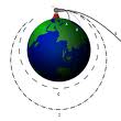
If the force is NOT constant, but proportional to distance (think swinging a cat round your head on its elastic tail!) we get interesting shapes:-


    '   ///////////////////   CentralForceKTimesExtn

    nomainwin

    UpperLeftX   =  10
    UpperLeftY   =   2
    WindowWidth  = 920
    WindowHeight = 650

    graphicbox #w.g1,  10,  10, 880, 480

    graphicbox #w.g3, 500, 510, 100, 100

    open "Motion under constant centripetal force plus k x extension." for window as #w

    #w,    "trapclose [quit]"

    global pi
    pi =3.1415923535

    k  =10   '   Hooke's Law, spring constant

    #w.g1, "down ; size 4 ; set 200 200 ; size 1; flush"

    #w.g3, "down ; backcolor red ; color red"

    vmax =10

    x           =   0                   '   initial horizontal position
    vx          =vmax

    y           =  18                   '   initial vertical height
    vy          =   0                   '   initial vertical velocity

    force1      =( vx^2 +vy^2) /15          '   exact circular orbit velocity. Try *0.9 or *1.2

    t           =   0                   '   initial time
    dt          =   0.01                '   time interval between updates

  [here]
    RadDist =( x^2 +y^2)^0.5

    theta   =atan2( y, x)
    print x, y, theta

    force   =force1 + ( RadDist -15) *k

    accny   =-1 *force *sin( theta)
    accnx   =-1 *force *cos( theta)

    vy      =vy +accny *dt
    y       =y     +vy *dt

    vx      =vx +accnx *dt
    x       =x     +vx *dt

    t       =t  +dt

    #w.g1, "set "; 200 +10 *x; " "; 200 -10 *y
    #w.g3, "cls ; home ; north ; turn "; 90 -theta *180 /pi; " ; circle 30 ; size 2 ; go -30"
    scan

    if RadDist >10 and RadDist <80 then goto [here]


    #w.g1, "flush"

    wait

function atan2( y, x)
    if x >0           then at =atn( y /x)
    if y >=0 and x <0 then at =atn( y /x) +pi
    if y <0  and x <0 then at =atn( y /x) -pi
    if y >0  and x =0 then at =    pi /2
    if y <0  and x =0 then at = 0 -pi /2
    if y =0  and x =0 then notice "undefined": end
    atan2 =at
end function

[quit]
    close #w
    end

Central repulsive forces

By making the force OUTWARD from a centre, and of strength prportional to R^-2, we can simulate alpha-scattering from a nucleus. It was the experimental observation of this, with far larger angles than expected, which proved the nuclear model of the atom with most of it being empty space. Only by getting within 1/1000 th of the atom radius could the observed deflections be explained- and in that 'outer region' could only be electron clouds..


    '   ///////////////////   CentralForceRepulsive


    nomainwin

    UpperLeftX   =  10
    UpperLeftY   =   2
    WindowWidth  = 920
    WindowHeight = 650

    graphicbox #w.g1,  10,  10, 880, 480

    graphicbox #w.g3, 500, 510, 100, 100

    open "Motion under constant centripetal force." for window as #w

    #w,    "trapclose [quit]"

    global pi
    pi =3.1415923535

    #w.g1, "goto 200 200 ; down ; backcolor lightgray ; circlefilled 160 ; size 3 ; set 200 200 ; size 1 ; flush"

    #w.g3, "down ; backcolor red ; color red"

    c           =   0

'for yy =-27 to 27 step 0.3
for i =1 to 1000
    x           = -20                   '   initial horizontal position
    y           =  -27 +55 *rnd( 1)     '   random incident height
    vx          =  50
    vy          =   0                   '   initial vertical velocity
    t           =   0                   '   initial time
    dt          =   0.001               '   time interval between updates
  [here]
    theta   =atan2( y, x)
    force   =(( x^2 +y^2)^-1) *1000
    accny   =1 *force *sin( theta)
    accnx   =1 *force *cos( theta)
    vy      =vy +accny *dt
    y       =y     +vy *dt
    vx      =vx +accnx *dt
    x       =x     +vx *dt
    t       =t  +dt

    '#w.g1, "color "; c; " 40 "; 255 -c
    #w.g1, "set "; 200 +10 *x; " "; 200 -10 *y
    #w.g3, "cls ; home ; north ; turn "; 90 -theta *180 /pi; " ; circle 30 ; size 2 ; go -30"
    scan
    if ( x^2 +y^2) <4900 then goto [here]
    'c =c +1
next i'next yy

    #w.g1, "flush"

    wait

function atan2( y, x)
    if x >0           then at =atn( y /x)
    if y >=0 and x <0 then at =atn( y /x) +pi
    if y <0  and x <0 then at =atn( y /x) -pi
    if y >0  and x =0 then at =    pi /2
    if y <0  and x =0 then at = 0 -pi /2
    if y =0  and x =0 then notice "undefined": end
    atan2 =at
end function

[quit]
    close #w
    end

Central forces- Newton's 'gedanken experiment'.

Many interesting case -eg orbits- are most easily handled by using polar coordinates. This nicely covers things like orbits. Newton was the first to consider this- with the example of a cannon, fired faster and faster horizontally at the top of a high mountain, above most of the atmosphere.